Since it was published in 2024, Alex Cheddar’s book Find the Fox: the Almost Impossible Word Search has become quite popular for its difficulty and novelty. If you haven’t heard of this book, the concept is very simple: it’s a word search where the grid consists solely of the letters $\F$, $\O$, and $\X$. There’s only one word to find: FOX, which appears once among all 200 pages of the book. As is standard in word searches, the string can appear horizontally, vertically, or diagonally, and either forward or reversed. Here’s the first page of the book, extracted from the Amazon preview:

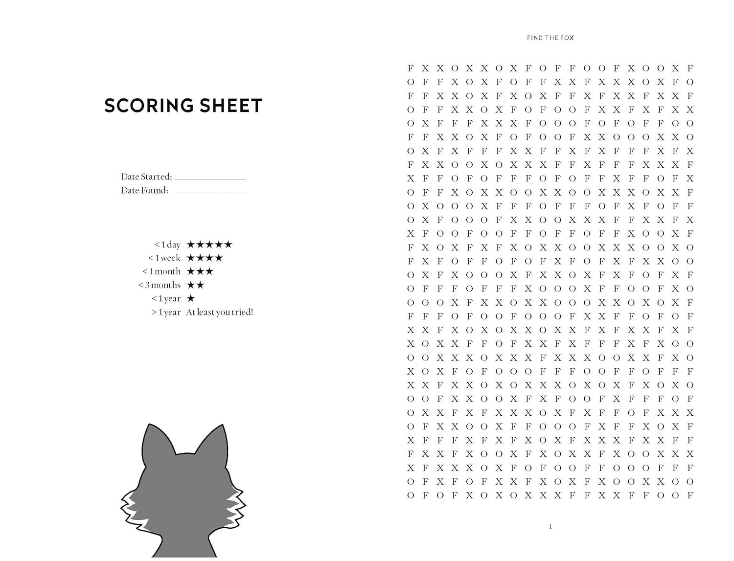
Upon a quick inspection, the letters seem to be fairly uniformly distributed – conditional, of course, on the string FOX not appearing (it’s definitely not on this page). This led me to think about how the book would have been generated (I certainly hope that Mr. Cheddar didn’t write the book¹ manually, letter by letter). Each of the 200 pages consists of a $32 \times 20$ grid. Assuming the letters really are randomly generated, the book can be said to have been sampled from the $\mathrm{Unif}(\{\F,\O,\X\}^{32 \times 20 \times 200})$ distribution conditional on the string $\FOX$ only appearing once. Sampling from this conditional distribution is not trivial. In this post, we’ll develop a method to do so using MCMC.

First of all, we can probably agree that any reasonable method will first sample from the distribution in which the string doesn’t appear anywhere, and then randomly choose a spot to insert it. The essential strategy behind the last part is fairly straightforward: we simply overwrite some $3$-letter string to $\FOX$, and then ensure that we haven’t inadvertently created additional $\FOX$s in the process. So for now, let’s focus on generating a single $\FOX$-less grid. Call a grid $\FOX$less if it doesn’t contain the string $\FOX$ anywhere, and let $\Omega$ be the set of $\FOX$less $32 \times 20$ grids. We want to sample from the $\text{Unif}(\Omega)$ distribution, which we’ll call $\pi$ (as per tradition).

Exact Sampling

In principle, the simplest way to sample from $\pi$ is by rejection sampling: that is, we keep sampling from $\mathrm{Unif}(\{\F,\O,\X\}^{32 \times 20})$ distribution until we produce a grid in $\Omega$. The only challenge here is coding up a $\FOX$less grid checker, which is more of a programming exercise than anything else. Here’s a way to do it:

import random

letters = ("F", "O", "X")
height, width = 32, 20

# 8 directions (dx, dy)
dirs = [(0,1), (1,0), (1,1), (1,-1),
        (-1,0), (0,-1), (-1,1), (-1,-1)]

def in_bounds(r, c):
    return 0 <= r < height and 0 <= c < width

def violates_local(grid, r, c, directions):
     # check whether FOX appears in any 3-cell segment that includes (r,c), along any direction
    for dr, dc in directions:
        # the triple can be (r-2dr,r-dr,r), (r-dr,r,r+dr), or (r,r+dr,r+2dr)
        for offset in (-2, -1, 0):
            coords = [(r + (offset + k)*dr, c + (offset + k)*dc) for k in range(3)]
            if all(in_bounds(rr, cc) for rr, cc in coords):
                triple = tuple(grid[rr][cc] for rr, cc in coords)
                if triple in (letters, letters[::-1]):
                    return True
    return False

def is_FOXless(grid):
    # full scan
    for r in range(height):
        for c in range(width):
            if violates_local(grid, r, c, dirs):
                return False
    return True

The rejection sampler then follows:

random.seed(1729)

FOXlessgrid = False

while not FOXlessgrid:
  newgrid = [[random.choice(letters) for _ in range(width)] for _ in range(height)]
  FOXlessgrid = is_FOXless(newgrid)

print(newgrid)  

Because the proposal distribution is uniform over all $3^{32 \cdot 20}$ grids, the accepted sample is exactly uniform over the $\FOX$less ones. So in theory, this works! You can try running this if you want, but I wouldn’t recommend it. Why? The problem is the acceptance rate $p_\text{acc}$. Computing the exact acceptance rate is essentially an inclusion-exclusion/transfer-matrix counting problem which explodes combinatorially in $2$ dimensions, but we can compute a rigorous upper bound.

Let $N$ be the number of length-$3$ segments we’re checking. Checking for a $\FOX$less grid is equivalent to checking the four “forward” directions (→, ↓, ↘, ↙) — of which there are

segments — for the presence of the strings $\FOX$ and $\XOF$. For each segment, we’re forbidding $2$ out of $3^3$ patterns, so the probability that a single segment is forbidden is $2/27$. The expected number of forbidden segments in a random grid is then $2256 \cdot (2/27) = 167.1111\ldots$. For a quick upper bound on the acceptance probability, we can consider only disjoint segments. In each row of length $20$ we can choose $6$ disjoint horizontal triples (covering $18$ cells), which across $32$ rows comes to $192$ independent triples. If the grid is $\FOX$less, then none of these triples can be $\FOX$ and $\XOF$, and hence

So the acceptance rate is at most about one in 2.6 million, which doesn’t seem horrible if we’re running our code on a peppy, multithreaded processor and we’re willing to wait for a few days. In fact, this bound is misleadingly optimistic — it overstates the probability by a factor of over 230 quadrillion.

To show this, we can invoke Janson’s inequality,² which provides exponential upper bounds on the probability that none of a large collection of weakly dependent “bad” events occur, in terms of their expected count and the sum of their pairwise dependencies. Let $A_i$ be the event that segment $i$ is $\FOX$ or $\XOF$. Then the events $A_i$ and $A_j$ are independent unless the segements $i$ and $j$ share at least one cell. Define

where $i \sim j$ means that segments $i$ and $j$ overlap and $m$ is the number of overlapping pairs of segments. The probability that we want is $p_\text{acc} = \P(X = 0)$, which, according to Janson’s inequality,³ satisfies

How can we compute $\mu$ and $\Delta$? Observe that $\mu$ is simply the expected number of forbidden segments in the random grid, which we computed above as $167.111\ldots$. To compute $\Delta$, note that for each pair $(i,j)$, there are $4$ pattern combinations:

For each combination, we have a set of letter constraints on the union of the cells used by the two segments. Because the letters are independent and uniform, if the constraints are inconsistent (i.e., the same cell is required to be both $\F$ and $\X$), then $\P(A_i \cap A_j) = 0$; otherwise, the union involves $m_{ij} \in \{4,5\}$ distinct cells and

We thus compute:

from collections import defaultdict
from itertools import combinations, product

# generate all length-3 segments
segments = [
    tuple((r + k*dr, c + k*dc) for k in range(3))
    for r in range(height) for c in range(width)
    for dr, dc in dirs[:4]
    if all(in_bounds(r + k*dr, c + k*dc) for k in range(3))
]

# index segments by cell
cell_to_segs = defaultdict(list)
for i, seg in enumerate(segments):
    for cell in seg:
        cell_to_segs[cell].append(i)

# get all overlapping segment pairs
pairs = {
    tuple(sorted(p))
    for idxs in cell_to_segs.values()
    for p in combinations(idxs, 2)
}

# compute probability that two segments are both FOX/XOF
def pair_prob(s1, s2):
    total = 0.0
    for p1, p2 in product((letters, letters[::-1]), repeat=2):
        req = {}
        ok = True
        for (cell, ch) in zip(s1, p1):
            if cell in req and req[cell] != ch:
                ok = False; break
            req[cell] = ch
        for (cell, ch) in zip(s2, p2):
            if cell in req and req[cell] != ch:
                ok = False; break
            req[cell] = ch
        if ok:
            total += 3 ** (-len(req))
    return total

Delta = sum(pair_prob(segments[i], segments[j]) for i, j in pairs)
print(Delta)

This gives $\Delta \approx 171.4567$. Hence $p_\text{acc} \leq e^{-54.7545} \approx 1.6613 \times 10^{-24}$. Conclusion: don’t use the rejection sampler.

There’s another way to sample exactly from our target distribution, this time using a bit of dynamic programming. To start off, define a scanning order (say row-by-row). At each step, to choose the next letter uniformly, we count how many completions exist if we put $\F$ here, how many exist if we put $\O$, and how many exist if we put $\X$. Then we sample from the three letters with probabilities proportional to those completion counts. Seems simple enough! The catch is that for length-$3$ strings in $8$ directions, whether a choice is $\FOX$less depends on a “neighborhood” of “radius” $2$, and the state we need to remember while sweeping is essentially the previous two rows (across their full widths), plus the last two letters of the current row we’re moving across. The number of states is on the order of $3^{2w}$, where $w$ is the width of the grid. For $w = 20$, it’s hopeless.⁴

Approximate Sampling

Instead of trying to sample from $\pi$ directly, what if we start off with some $\FOX$less grid, and then modify it so that it looks like it came from $\pi$? This is where we can exploit MCMC. We will define a symmetric random walk on $\Omega$, where each step makes a tiny local random change but does not violate the constraint. Generating a $\FOX$less grid (call it $G_0 \in \Omega$) is easy for initialization purposes: for example, the grid consisting entirely of $\F$s is perfectly $\FOX$less. Let’s now construct our Markov chain. At the $t$th iteration of our sampler, we’ll do the following:

1. Choose a cell $(i,j)$ in $G_t$ uniformly at random
2. Propose changing the letter in that cell to one of the other two letters (chosen uniformly)
3. If the resulting grid is still $\FOX$less (i.e., we didn’t create a new $\FOX$), then accept the move and call the new grid $G_{t+1}$; otherwise, reject the proposed change and set $G_{t+1} = G_t$

The resulting chain $\{G_t\}_t$ is obviously time-homogenous. But is $\pi$ really stationary for this Markov chain? Let $G, G’ \in \Omega$ differ in exactly one cell (say the $k$th), and suppose that changing the cell from letter $a$ to letter $b$ keeps the grid $\FOX$less. The probability of moving from $G$ to $G’$ is

and the probability of the reverse move is exactly the same. Since $\pi(G) = 1/\lvert\Omega\rvert$ for any $G \in \Omega$, we have

So the detailed balance condition is satisfied, and $\pi$ is indeed stationary for our Markov chain.

What about aperiodicity? If we form a graph $\mathcal{G}$ whose vertices are grids in $\Omega$ and draw an edge between vertices $G$ and $G’$ if and only if the grids differ in exactly one cell, then we can view our algorithm as a random walk on $\mathcal{G}$. A random walk on an undirected graph is aperiodic if and only if the graph is non-bipartite, and for $\mathcal{G}$ to be non-bipartite, it suffices to find an odd cycle. But that’s easy! Start from the all-$\F$ grid, then change the first cell to an $\O$, then to an $\X$, and then to an $\F$. All of these grids are clearly in $\mathcal{G}$, so we’ve exhibited a cycle of length $3$ (i.e., a triangle), and our Markov chain is aperiodic.

The only tricky bit is irreducibility. In order to guarantee that the law of $G_t$ will actually converge to $\pi$ as $t \to \infty$, we need to show that our chain is irreducible: any $\FOX$less grid should be reachable from any other via $\FOX$less single-cell flips. Equivalently, we need to show that $\mathcal{G}$ is connected. Fortunately, with some care we can prove this. To be general, we’ll prove the result for any grid size.

For some setup, fix integers $h,w \geq 1$ and identify grid cells with coordinates $(r,c)$ where $r \in \{1,\ldots,h\}$ and $c \in \{1,\ldots,w\}$. A length-$3$ line segment is any triple of distinct cells of the form

where

and all three cells lie in the grid. Define a $\FOX$less single-cell flip to be an operation that changes the letter in exactly one cell and results in another grid in $\Omega$. We order the cells in row-major order: $(r,c) \prec (r’,c’)$ if either $r < r’$ or $r = r’$ and $c < c’$. Let $C_1, C_2, \ldots, C_{hw}$ denote the cells in this order. $G(C_i)$ refers to the letter in the $i$th cell of $G$.

Proposition: For every $G \in \Omega$, there exists a sequence of $\FOX$less single-cell flips that transforms $G$ into the all-$\O$ grid. Consequently, $\mathcal{G}$ is connected.

Proof: We will explicitly construct a $\FOX$less path from an arbitrary $G \in \Omega$ to the all-$\O$ grid. We process cells in row-major order. For $i = 1, 2,\ldots, hw$, at step $i$ we change the value of cell $C_i$ to $\O$ if it’s not already $\O$. Fix $i$ and let $G^{(i)}$ denote the grid after step $i$, with $G^{(0)} := G$. It is immediate that $G^{(i)}(C_j) = O$ for all $j \leq i$ (i.e., this is an invariant). We will show by induction that $G^{(i)} \in \Omega$. We already know that $G^{(0)} \in \Omega$, so suppose that $G^{(i-1)} \in \Omega$ and consider the transition $G^{(i-1)} \to G^{(i)}$, where we set $C_i$ to $\O$. Any newly created forbidden pattern $\FOX$ or $\XOF$ would need to involve $C_i$, since all other cells are unchanged. Moreover, $\O$ must appear in the middle of such a triple. Therefore, if setting $C_i$ to $\O$ creates a forbidden pattern, then $C_i$ must be the center cell of some length-$3$ line segment whose two opposite neighbors have labels $\F$ and $\X$ in $G^{(i)}$.

It thus suffices to show that after the update, $C_i$ cannot have opposite neighbors $\F$ and $\X$ along any of the four lines through $C_i$ (horizontal, vertical, and the two diagonals). Let $C_i = (r_i, c_i)$. Consider any pair of opposite neighbors of $C_i$ along a line segment of length $3$ (when such neighbors exist within the grid). These opposite pairs are:

• Horizontal: $(r_i, c_i-1)$ and $(r_i, c_i+1)$
• Vertical: $(r_i-1, c_i)$ and $(r_i+1, c_i)$
• Diagonal NW-SE: $(r_i-1, c_i-1)$ and $(r_i+1, c_i+1)$
• Diagonal NE-SW: $(r_i-1, c_i+1)$ and $(r_i+1, c_i-1)$

In every case, one of these two neighbors either lies in a strictly earlier row than $C_i$, or in the same row but an earlier column. Concretely:

• In the horizontal pair, $(r_i, c_i-1) \prec (r_i,c_i)$
• In the vertical pair, $(r_i-1, c_i) \prec (r_i,c_i)$
• In the diagonal NW-SE pair, $(r_i-1, c_i-1) \prec (r_i,c_i)$
• In the diagonal NE-SW pair, $(r_i-1, c_i+1) \prec (r_i,c_i)$

Thus, whenever a length-$3$ segment centered at $C_i$ exists, at least one of the two opposite neighbors is some $C_j$ with $j < i$. By the induction invariant applied at step $i-1$, that neighbor is already $\O$ in $G^{(i-1)}$, and it remains $\O$ in $G^{(i)}$ since we only changed $C_i$. Therefore, in $G^{(i)}$ every existing opposite-neighbor pair around $C_i$ contains at least one $\O$. In particular, it is impossible for the two opposite neighbors to be $\F$ and $\X$ (in some order). Hence no forbidden pattern can be centered at $C_i$, and so setting $C_i$ to $\O$ cannot create a forbidden pattern. We conclude that the move $G^{(i-1)} \to G^{(i)}$ is $\FOX$less; that is, $G^{(i)} \in \Omega$. This completes the induction step. After $hw$ steps, every cell has been set to $\O$, so $G^{(hw)}$ is the all-$\O$ grid. This proves that every $G \in \Omega$ can be transformed to the all-$\O$ grid through a sequence of $\FOX$less single-cell flips.

Now, take any two grids $G, G’ \in \Omega$. By the previous construction, there exists a $\FOX$less path from $G$ to the all-$\O$ grid, and likewise from $G’$ to the all-$\O$ grid. Reversing the second path gives a $\FOX$less path from the all-$\O$ grid to $G’$, and concatenating the first path and the reversed second path yields a $\FOX$less path from $G$ to $G’$. Thus $\mathcal{G}$ is connected. $\square$

So our Markov chain is irreducible and aperiodic, and therefore has a unique stationary distribution. Since $\pi$ is stationary (as we verified from the detailed balance condition), it is the unique stationary distribution, and for any starting state $G_0 \in \Omega$, we have $\mathcal{L}(G_t) \to \pi$ as $t \to \infty$ by the standard finite-state Markov chain convergence theorem.

It remains to actually code up our sampler. We’ll go for $1{\small,}100{\small,}000$ iterations, burn off the first $50{\small,}000$ and thin every $50{\small,}000$th sample. These numbers may seem large compared to what you’d often see in simpler applications (especially in continuous-space settings), but remember that our Markov chain transitions are local moves in an enormous, heavily constrained state space, so mixing is necessarily slow: changing the large-scale features of a grid requires a lot of accepted local moves, so we’ll need a lot of iterations before the chain forgets its initialization and reaches more typical configurations. We thin aggressively because successive states of the chain are highly correlated; each iteration proposes a change at a single cell, so even accepted moves alter only one of $32 \times 20 = 640$ cells. As a result, many iterations are required before the chain produces a meaningfully different grid, and large thinning factor gives us approximately independent-looking samples; similarly, a large burn-in period allows us to confidently move past the all-$\F$ initialization grid.

def step(grid, lazy_p=0.5):
    r = random.randrange(height)
    c = random.randrange(width)
    old = grid[r][c]
    new = random.choice([x for x in letters if x != old])

    grid[r][c] = new
    if violates_local(grid, r, c, dirs[:4]):  # reject if we created a forbidden triple
        grid[r][c] = old

def run_chain(steps=1_100_000, burn=50_000, thin=50_000, seed=None):
    if seed is not None:
        random.seed(seed)

    # start from an easy $\FOX$less state (all F)
    grid = [["F"] * width for _ in range(height)]

    snapshots = []
    for t in range(1, steps + 1):
        step(grid)

        if t >= burn and (t - burn) % thin == 0:
            snapshots.append(["".join(row) for row in grid])

    return snapshots


pages = run_chain(seed=1729)
print("\n".join(pages[0][:10]))

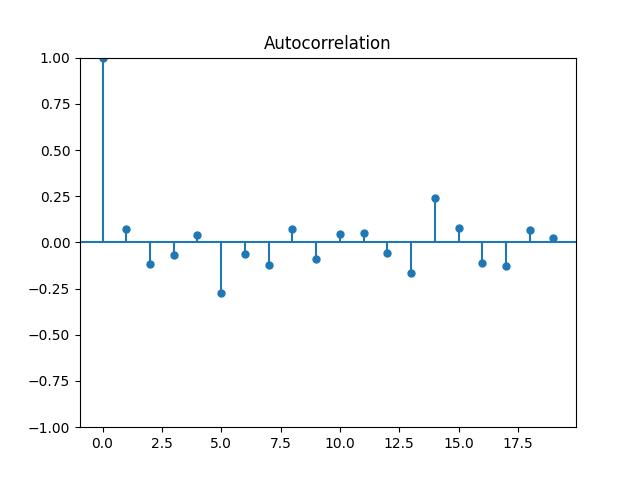
This takes about 10 seconds to run and produces 20 grids. Some quick MCMC diagnostics: our acceptance rate is a healthy $0.452$, and some acf plots suggest that the autocorrelation of the resulting samples decays reasonably fast:

Each acf above was based on a time series of summary statistics computed from the grids. The first time series ${D^{(1)}_t}$ is the Hamming distance between the $t$th sampled grid and the all-$\F$ grid, \(D^{(1)}_t = |\{c \in \{1,\ldots,h\} \times \{1,\ldots,w\}: G_t(c) \neq G^*(c)\}|, \notag\) while the second ${D^{(2)}_t}$, is an average of six single-cell indicators for the letter $\X$, \(\{D^{(2)}_t\} = \frac{1}{6} \sum_{j=1}^g \one{G^t(c_j) = \X}, \notag\) where the cells $c_1, \ldots, c_6$ were randomly selected. Both of these summary statistics are sensitive to structural features: the Hamming distance measures how much the configuration of letters has changed as a whole, while the single-cell $\X$-indicators reflect local changes.

The frequencies of the letters $\F$, $\O$, and $\X$ at the last sampled grid are $0.323$, $0.328$, and $0.348$ respectively, which is about what we’d expect. More precisely, each of those is the observed value of the pushforward of $\pi$ under the coordinate projection onto a single cell. The unconditional distribution $\text{Unif}(\{\F,\O,\X\}^{32 \times 20})$ is invariant under any permutation of the letters, but the conditioning event “no $\FOX$ appears” is not: it’s invariant under the swap $\F \leftrightarrow \X$ but not under permutations involving $\O$, since $\O$ is singled out as the middle letter of the forbidden pattern. It follows that $\pi(\F) = \pi(\X)$. On the other hand, there’s no symmetry that forces $\pi(\O)$ to equal the common value of $\pi(\F)$ and $\pi(\X)$; nevertheless, we’d expect it to be reasonably close. Determining the exact values (either for a finite $h \times w$ grid or for the infinite-grid limit) is a very difficult combinatorial problem and not worth the trouble.

Inserting a FOX

Now, finally, what about putting in a $\FOX$? To do this, we can simply sample one of our grids (uniformly at random) and then change a $3$-letter segment to $\FOX$.⁵ The harder part is ensuring that this doesn’t accidentally create another $\FOX$ nearby via overlapping triples. To do this, we’ll construct a function that picks a random $3$-letter segment uniformly from the grid, and then overwrites it with either $\FOX$ or $\XOF$ (with equal probability). Now, observe that if an arbitrary $3$-letter segment in the grid doesn’t touch any changed cell, then its three letters are exactly the same as before, so it couldn’t suddenly become $\FOX$ if it wasn’t already. Thus, if there are other $\FOX$s after the overwrite, we know that they must be among the length-$3$ segments that intersect the cells that we changed. So we need only enumerate those segments, of which there are a constant number. If, among those segments, we count more than one $\FOX$, we undo the overwrite and try again with another random segment.

Somewhat counterintuitively, most random overwrites of $\FOX$ won’t actually create extra $\FOX$s, because to do so requires a fairly specific local coincidence: the overwritten letters must also complete another length-$3$ pattern passing through one of the modified cells. Since we only alter $3$ cells, the “impact radius” is small, so the probability of collateral $\FOX$s is small as well. You can try this with the first page of Find the Fox above: try to pick any length-$3$ segment at random,⁶ change the letters to $\FOX$, and see if that change created any extra $\FOX$s. Chances are that it didn’t!

It’s worth noting that this method does introduce a tiny amout of sampling bias. This is because when we take a valid 1-$\FOX$ grid $H$ and work backwards, it must have been arisen from a $\FOX$less grid $G \in \Omega$ together with a segment $s$ such that overwriting $s$ with $\FOX$ or $\XOF$ produces $H$ without creating different $\FOX$/$\XOF$ occurences. However, different 1-$\FOX$ grids admit different numbers of such “preimages” $(G,s)$, depending on the cells surrounding $s$. 1-$\FOX$ grids in which the letters surrounding $\FOX$ restrict those valid preimages are slightly less likely to be produced. In other words, our procedure samples 1-$\FOX$ grids with probability proportional to the number of $\FOX$less configurations that lead to them, rather than uniformly. But practically speaking, the difference seems to be negligible.

segments = []

for r in range(height):
    for c in range(width):
        for dr, dc in dirs[:4]:  # →, ↓, ↘, ↙
            coords = [(r + k*dr, c + k*dc) for k in range(3)]
            if all(in_bounds(rr, cc) for rr, cc in coords):
                segments.append((tuple(coords), (dr, dc)))

def segments_through_cell(r, c):
    # all length-3 segments (4 directions) that include (r,c)
    out = []
    for dr, dc in dirs[:4]:
        for off in (-2, -1, 0):
            coords = [(r + (off+k)*dr, c + (off+k)*dc) for k in range(3)]
            if all(in_bounds(rr, cc) for rr, cc in coords):
                out.append(tuple(coords))
    return out

def count_fox_in_affected(grid, affected_cells):
    # count FOX/XOF occurrences among segments that intersect affected_cells
    seen = set()
    total = 0
    for (r, c) in affected_cells:
        for seg in segments_through_cell(r, c):
            if seg in seen:
                continue
            seen.add(seg)
            triple = tuple(grid[rr][cc] for rr, cc in seg)
            if triple in (letters, letters[::-1]):
                total += 1
    return total

def inject_exactly_one_fox(grid, max_tries=200000):
    for _ in range(max_tries):
        (cells, (dr, dc)) = random.choice(segments)
        pat = random.choice((letters, letters[::-1]))  # choose FOX or XOF orientation on this segment

        new = [row[:] for row in grid]
        changed = []
        for (rr, cc), ch in zip(cells, pat):
            if new[rr][cc] != ch:
                new[rr][cc] = ch
                changed.append((rr, cc))

        # if we didn't change anything, we'd still have 0 occurrences — skip
        if not changed:
            continue

        # starting grid has 0; any new occurrence must touch a changed cell
        if count_fox_in_affected(new, changed) == 1:
            return new, {"cells": cells, "dir": (dr, dc), "pattern": pat}

    raise RuntimeError("Failed to inject exactly one FOX; increase max_tries.")

Finally, we can create a fresh “book” with as many pages as we’d like. For example, you might like the idea of Find the Fox but think that 200 pages is a bit much. We can easily create a single page with exactly one $\FOX$ in it! And once we solve that one, we can create another one (and continue ad nauseam until we get bored of finding foxes, which I imagine won’t take very long). The code for generating the PDF isn’t very interesting so I’ll omit it here, but a command-line interface is available at https://github.com/rob-zimmerman/find-the-fox-mcmc with a number of useful options that you can specify (custom alphabet, grid height and width, number of pages, MCMC controls, etc.) Here’s an example of a generated page, and here’s the solution key with the $\FOX$ coloured in red. Enjoy! If you liked this, please support the author and publisher of Find the Fox and purchase the book! Once you’ve solved it, come back here and generate an iid copy of the book and start again.

The Moment Problem

In probability theory, a rigorous definition of expectation is followed almost immediately by a proof of the law of the unconscious statistician; following that, one is shown the definition of moments. One encounters integer moments throughout probability and statistics, while non-integer moments are substantially rarer. A natural question that arises is whether a distribution is characterized by its integer moments. That is, given a sequence of real numbers $\{\mu_j\} _{j=1}^\infty$, is there (at most) one distribution $F$ with $\mu_p = \int x^p \, \mathrm{d}F$? This question is called a moment problem.

One learns by example that the answer is no, in general. Work on the moment problem reaches back to Stieltjes in 1894 (who himself invented the term moment), with precursors in Chebyshev and Markov.¹ Using the theory of continued fractions, Stieltjes himself solved the moment problem for distributions supported on $(0, \infty)$, ultimately showing that it relied on the positivity of the determinants of what we now call Hankel matrices built up from the prescribed moments (in the days before measure theory, Stieltjes’ moments were defined by what we know today as Riemann-Stieltjes integrals). The standard counterexample came in 1963, when Chris Heyde asked about the moment problem for “commonly used distributions in statistics” and presented the famous log-normal family:²

Example 1: Let $\mu \in \R$ and $\sigma^2 > 0$. If $X$ is a $\text{Lognormal}(\mu, \sigma^2)$ random variable — that is, if $X$ has density $f(x) = \frac{1}{\sqrt{2\pi}\sigma x} \exp\left(-\frac{(\log(x) - \mu)^2}{2\sigma^2}\right)$ for $x \in \R$ — then for all $\varepsilon \in [-1,1]$, the function $f \cdot (1 + \varepsilon \cdot \sin(2\pi \log{x}))$ is also a density with the same moments as $X$.

According to Stoyanov³, Stieltjes himself showed this for the $\text{Lognormal}(0, 1)$ case in the same 1894 paper as his “moment” introduction (in a non-probabilistic context, of course), so Heyde’s example was apparently something of a rediscovery. Durrett⁴ gives us another example:

Example 2: Let $\lambda \in (0,1)$. If $X$ has density $f(x) = \left(\int \exp(-|x|^\lambda) \, \mathrm{d}x \right)^{-1} \exp\left(-|x|^{\lambda}\right)$ for $x \in \R$, then for all $\varepsilon \in [-1,1]$, the function $f \cdot (1 + \varepsilon \cdot \sin( \tan(\lambda \pi /2) \cdot |x|^\lambda \cdot \mathrm{sgn}(x)))$ is also a density with the same moments as $X$.

Examples 1 and 2 obviously share a similar theme. It turns out that the idea generalizes to Stieltjes classes:³ if $f$ is a density whose integer moments exist and $h$ is a non-zero continuous function taking values in $[-1,1]$ such that $\E_{X \sim f}[h(X) \cdot X^n] = 0$ for all $n \in \N$, then for all $\varepsilon \in [-1,1]$, the function $f_\varepsilon = f \cdot (1 + \varepsilon \cdot h)$ is a density with the same moments as $f$. The conditions required of $h$ essentially forces it to be periodic, as it is in the two examples above.

Non-Integer Moments

Going through the explicit proofs of Examples 1 and 2 in Durrett’s book, I was struck that the equivalance of the moments ultimately relies on the fact that we’re really talking about integer moments here (in Example 1, the integers play into the sine function; in Example 2, they essentially make $x^n \cdot \varepsilon \cdot h \cdot f$ into an odd function that integrates to $0$). Clearly, non-integer moments are a different story. This observation led me to a kind of inverse question: does there exist a distribution which is determined only by its non-integer moments? To put it another way, for $p \in \R$, do there exist positive random variables $X$ and $Y$ such that $\E[X^p] = \E[X^p]$ if and only if $p \not \in \N$? The answer, as it turns out, is no. In fact, we only need the moments to coincide on some dense subset of $\R$ such as the rationals:

Proposition: Let $X$ and $Y$ be positive random variables. If $A \subseteq \R$ is dense in $\R$ and $\E[X^p] = \E[Y^p]$ for all $p \in A$, then $\E[X^p] = \E[Y^p]$ for all $p \in \R$.

Proof: Fix $p \in \R$. We have two cases to consider: either $\E[X^p] = \infty$ or $\E[X^p] < \infty$. The first case is fairly easy to handle, while the second is only a bit trickier.

Case 1: $\E[X^p] = \infty$.

Fix a sequence $\{q_j\}_{j=1}^\infty$ such that $q_j \to 0$ and $p + q_j \in A$ for all $j$ (we can do this because $A$ is dense in $\R$). We have that

Thus $\E[Y^p] = \infty$, which gives $\E[X^p] = \E[Y^p]$.

Case 2: $\E[X^p] < \infty$.

To begin with, let’s show that $\E[Y^p] < \infty$ using essentially same technique as we used above, but in the contrapositive direction. Fix another sequence $\{r_j\}_{j=1}^\infty$ such that $r_j \to 0$ and $p - r_j \in A$ for all $j$. Then

Now, let $\{p_j\}_{j=1}^\infty \subseteq A$ be a yet another sequence with $p_j \nearrow p$ as $j \to \infty$. Observe that for any $j \in \N$, we have

Since $\E[1 + X^p] < \infty$, we see that the $X^{p_j}$ are dominated by an integrable random variable. By the dominated convergence theorem, we get $\E[X^{p_j}] \to \E[X^p]$ as $j \to \infty$. The exact same argument applied to the $Y^{p_j}$ shows us that $\E[Y^{p_j}] \to \E[Y^p]$ as $j \to \infty$. Since $\E[X^{p_j}] = \E[Y^{p_j}]$ for all $j$, the uniqueness of limits (in metric spaces!) gives $\E[X^p] = \E[Y^p]$. $\square$

Taking $A = \R^{\geq 0} \setminus \N$ resolves the original question.

Back to the Moment Problem

The condition $\E[X^p] = \E[Y^p]$ for all $p \in \R$ is very strong. But is it enough to force $X$ and $Y$ to have the same distribution? The answer is yes!

Theorem 1: Let $X$ and $Y$ be positive random variables. If $A \subseteq \R$ is dense in $\R$ and $\E[X^p] = \E[Y^p] < \infty$ for all $p \in A$, then $X \stackrel{d}{=} Y$.

The proof follows along the same lines as that of a stronger theorem of Gwo Dong Lin from 1992:⁵

Theorem 2: Let $X$ and $Y$ be positive random variables, and suppose there exists some $\alpha > 0$ such that $\E[X^\alpha]$ and $\E[Y^\alpha] < \infty$. Let $\{s_j\}_{j=1}^\infty \subseteq (0, \infty)$ be a sequence of distinct numbers such that $s_j \to s \in (0, \alpha)$. If $\E[X^{s_j}] = \E[Y^{s_j}]$ for all $j$, then $X \stackrel{d}{=} Y$.

Clearly Theorem 1 is weaker than Theorem 2, so it’s enough to prove the latter; the former then falls out as a corollary. Lin’s proof is quite slick. Here’s a sketch of it:

Proof of Theorem 2 (sketch): The assumptions imply that the moment generating functions (mgs) of $\log{X}$ and $\log{Y}$ viewed as functions over $\C$ — that is, the functions $z \mapsto \E[X^z]$ and $z \mapsto \E[Y^z]$ — are analytic in the strip $S = \{z \in \C: 0 < \Re(z) < \alpha\}$ (because $\E[X^\alpha], \E[Y^\alpha] < \infty$), and moreover these functions, which are analytic continuations of their respective mgfs, agree on $S$ (because the equality of moments assumption activates the identity theorem). A (right)-continuity argument then shows that these functions agree on $\{z \in \C: \Re(z) = 0\}$ as well. Replacing $z$ with $it$ for $t \in \R$, we see that the characteristic functions of $\log{X}$ and $\log{Y}$ agree everywhere. From Lévy’s inversion theorem, we get that $\log{X} \stackrel{d}{=} \log{Y}$, and thus $X \stackrel{d}{=} Y$. $\square$

Let $X_0$ be supported on some nonempty $A \subseteq \N_{>0}$ with $\P(X_0 = k) = p_{0,k}$ and $\E[X_0] < \infty$. For each $n \geq 1$, recursively define $X_n$ on $\N_{>0}$ by $\P(X_n = k) = c_n \cdot k \cdot p_{n-1,k}$, where $c_n$ is a normalizing constant. Then, as $n \to \infty$,

…then what? What happens to these random variables in the pointwise limit? I remember asking myself this years ago when I first learned about discrete random variables, and, given the simplicity of the formulation, I was surprised when a search for an answer yielded nothing.

Anyway, the answer I tweeted was perhaps somewhat unsatisfying. This post is an attempt to do a little better.

Of course, the normalizing constant here is simply $\left(\sum_{k \in A} k \cdot p_{n-1,k} \right)^{-1} = \E[X_{n-1}]^{-1}$. So one way to look at this construction is to view the mass that $X_n$ places on $k$ as the corresponding (normalized) summand in the expectation of $X_{n-1}$. Observing that $p_{1,k} = \E[X_0]^{-1} \cdot k \cdot p_{0,k}$, we might suspect that this identity holds more generally provided that all moments exist,¹ and in fact an easy induction argument shows this is true:

Proposition: For all $n \geq 1$, we have $p_{n,k} = \E[X_0^n]^{-1} \cdot k^n \cdot p_{0,k}$, provided that $\E[X_0^n] < \infty$.

Proof: The base case $n=1$ is obvious. Now, assume that $p_{n-1,k} = \E[X_0^{n-1}]^{-1} \cdot k^{n-1} \cdot p_{0,k}$. Then, simply plugging this in, cancelling out normalizing constants and manipulating gives us

as desired. $\square$

We now return to the original question: what can we say about $X_n$ as $n \to \infty$? The answer to this, as it turns out, depends solely on whether $A$ is infinite or not. If $A$ is infinite, then for any fixed $k \in A$ we have

That is, $\P(X_n = k) \xrightarrow{n \to \infty} 0$. Observe that that this works because

which follows from our assumption that $A$ is infinite. Thus, for any fixed $k \in A$ we have $\P(X_n \leq k) \xrightarrow{n \to \infty} 0$, or equivalently $\P(X_n > k) \xrightarrow{n \to \infty} 1$, and we see that $X_n$ does not converge to a random variable as $n \to \infty$.

If $A$ is finite, then the situation is quite different. In this case, let $k^* = \max A$. Then we find that

That is, $\P(X_n = k^* ) \xrightarrow{n \to \infty} 1$. We can also see this with an approach from the other direction. For any $k \in A$ with $k < k^* $, we return to the situation of $\eqref{eq:ineq}$:

While the second sum in the parentheses is finite this time, we can be sure it’s non-empty because it must include a term for $k^*$ (the inequality is not strict this time!).

We can summarize our answer to the silly tweet question in a neat statement:

Theorem: Let $X_0$ be supported on some non-empty $A \subseteq \N^{>0}$ with $\P(X_0 = k) = p_{0,k}$ and $\E[X_0^n] < \infty$ for all $n \in \N$. For each $n \geq 1$, recursively define $X_n$ on $\N^{>0}$ by $\P(X_n = k) = c_n \cdot k \cdot p_{n-1,k}$, where $c_n$ is a normalizing constant. Then, as $n \to \infty$, the following holds:

1) If $|A| = \infty$, then $X_n$ does not converge.
2) If $|A| < \infty$, then $X_n$ converges to a point mass at $\max A$.

The first assessment in that course (in the form of an open-book online quiz — this was during lockdown, after all) was intended to test the students’ understanding of these concept; with lots of difficulty, I managed to come up with several original questions. One of them was meant to be on the trickier side:

Let $X_1,\ldots,X_n \stackrel{iid}{\sim} F_\theta$, where the $X_i$’s have finite first moments. Suppose that there exist some $j,k \in {1,\ldots,n}$ such that the statistic $S(\bX) = X_j$ is ancillary for $\theta$ and the statistic $T(\bX) = X_k$ is complete for the family $\{F_\theta: \theta \in \Theta\}$. Prove that all of the $X_i$’s must be constant with probability 1.

Solution: Let $h(T(\bX)) = T(\bX) - \E[X_j]$, which is free of $\theta$ because $X_j$ is ancillary for $\theta$. Then for any $\theta \in \Theta$, we have $\E[h(T(\bX))] = \E[X_k] - \E[X_j] = 0$, and by completeness it follows that $1 = \P_\theta( h(T(\bX)) = 0) = \P_\theta(X_k = \E[X_j])$ for all $\theta \in \Theta$. That is, $X_k$ is the constant $\E[X_j]$ with probability 1. Since the $X_i$’s are iid, they’re all equal to that same constant with probability 1. $\square$

The question originally had a number of red herrings thrown in, but fortunately I removed those before going live. In a subsequent discussion with pals Yanbo and Michaël, we noticed a connection to a basic result in probablity theory:

Theorem: A random variable $Y$ is independent of itself if and only if $Y$ is almost surely constant.

One direction of this is quite trivial. The other direction is substantially more difficult and is typically proved by appealing to Kolmogorov’s zero-one law (of course one easily shows that \(\P(Y \in A) \in \{0,1\}\) for any event \(A\) — perhaps specializing to \(\P(Y = y) \in \{0,1\}\) for any \(y \in \R\) — but clearly this is not enough to immediately conclude that \(\P(Y = y) = 1\) for some \(y \in \R\), and some topological argument is required). However, if we’re willing to further assume that $Y$ has a finite first moment, then we can produce an elementary proof using the result from the STA261 quiz:

$(\Rightarrow)$: Suppose that $Y$ is independent of itself. Define the “parameter space” $\Theta = \{ \theta \}$, where $\theta \in \R$ is arbitrary. We can vacuously associate $\theta$ to the distribution of $Y$ and write $Y \sim F_\theta$ without any ambiguity, even though the distribution of $Y$ is free of $\theta$. By the last remark, the “statistic” $S(Y) = Y$ is ancillary for $\theta$. Now, let $h: \R \to \R$ be some function such that $\E[h(Y)] = 0$. Since $Y$ is independent of itself, so too is $h(Y)$ and we have $0 = \E[h(Y)] \cdot \E[h(Y)] = \E[h(Y)^2]$, and it follows¹ that $\P(h(Y) = 0) = 1$, and this holds vacuously for all $\theta \in \Theta$. Thus, the “statistic” $T(Y) = Y$ is complete (and obviously sufficient) for the family $\{ F_\theta: \theta \in \Theta \}$. By the result from the quiz with $Y$ in place of each $X_i$, we see that $Y$ must be constant. $\square$

Unfortunately, this will not win the Most Elegant Proof award for that direction of the theorem under the assumption of a finite first moment: since $Y$ is independent of itself, $\E[Y^2] = \E[Y] \cdot \E[Y] = \E[Y]^2$ so that $\text{Var}(Y) = \E[Y^2] - \E[Y]^2 = 0$, and the result follows.